Audio spectrograms are a graphical representation of sound, showing how the energy of a signal is distributed across different frequencies over time. They are a useful tool in various fields such as speech processing, music analysis, and acoustic engineering. In this article, we will explore how to create an audio spectrogram using Python.
Required libraries
We will be using the following Python libraries to create our audio spectrogram:
- numpy: for numerical operations
- matplotlib: for visualization
- scipy: for signal processing
You can install these libraries using pip, the Python package manager:
pip install numpy matplotlib scipyOnce you have installed packages, we can start processing audio files.
Loading the audio file
To create a spectrogram, we first need to load an audio file. For this example, we will be using a WAV file. We can load the file using the scipy library as follows:
from scipy.io import wavfile

# Load the WAV file
sample_rate, samples = wavfile.read('audio.wav')
The sample_rate variable contains the sampling rate of the audio file, while samples is a one-dimensional array containing the audio data.
Preprocessing the audio data
Before we can create a spectrogram, we need to preprocess the audio data. First, we need to convert the one-dimensional array of audio data into a two-dimensional array of frames. We can use the numpy library for this:
import numpy as np

# Convert the one-dimensional audio data into frames
frame_size = 2048
hop_size = 512
frames = np.array([samples[i:i+frame_size].astype(np.float64) for i in range(0, len(samples) - frame_size, hop_size)])
In this example, we are using a frame size of 2048 samples and a hop size of 512 samples. This means that we will be processing 2048 samples at a time, and we will be shifting the frame by 512 samples for each iteration.
Next, we need to apply a window function to each frame. A window function is a mathematical function that is applied to each frame to reduce the effect of spectral leakage. We can use the Hanning window, which is a commonly used window function, as follows:
window = np.hanning(frame_size)
frames *= window
Computing the spectrogram
Once we have preprocessed the audio data, we can compute the spectrogram. We can use the Fourier transform to convert the time-domain signal into the frequency-domain signal. We can then calculate the power spectrum, which is the squared magnitude of the Fourier transform. Finally, we can apply a logarithmic scale to the power spectrum to create a spectrogram.
# Compute the Fourier transform
spectrogram = np.abs(np.fft.rfft(frames, n=frame_size))

# Compute the power spectrum
power_spectrum = spectrogram ** 2

# Compute the logarithmic scale spectrogram
log_spectrogram = 10 * np.log10(power_spectrum)
In this example, we are using the fast Fourier transform (FFT) algorithm to compute the Fourier transform. We are also using the rfft function, which only computes the positive frequencies, since the audio signal is real-valued.
Visualizing the spectrogram
Finally, we can use the matplotlib library to visualize the spectrogram:
import matplotlib.pyplot as plt

# Create the spectrogram plot
plt.imshow(log_spectrogram.T, aspect='auto', origin='lower', cmap='jet')
plt.xlabel('Time')
plt.ylabel('Frequency')
plt.colorbar()
plt.show()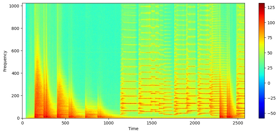
In this example, we are using the imshow function to display the spectrogram. We are setting the aspect parameter to 'auto', which automatically scales the plot to fit the figure size. We are setting the origin parameter to 'lower', which places the low frequencies at the bottom of the plot. We are using the 'jet' colormap to display the spectrogram, and we are adding a colorbar to the plot.
Full code
Here is the full code to create an audio spectrogram using Python:
from scipy.io import wavfile
import numpy as np
import matplotlib.pyplot as plt

# Load the WAV file
sample_rate, samples = wavfile.read('audio.wav')

# Convert the one-dimensional audio data into frames
frame_size = 2048
hop_size = 512
frames = np.array([samples[i:i+frame_size].astype(np.float64) for i in range(0, len(samples) - frame_size, hop_size)])

# Apply the Hanning window function to each frame
window = np.hanning(frame_size)
frames *= window

# Compute the spectrogram
spectrogram = np.abs(np.fft.rfft(frames, n=frame_size))
power_spectrum = spectrogram ** 2
log_spectrogram = 10 * np.log10(power_spectrum)

# Create the spectrogram plot
plt.imshow(log_spectrogram.T, aspect='auto', origin='lower', cmap='jet')
plt.xlabel('Time')
plt.ylabel('Frequency')
plt.colorbar()
plt.show()
In this article, we have explored how to create an audio spectrogram using Python. We used the numpy, matplotlib, and scipy libraries to load and preprocess an audio file, compute the spectrogram, and visualize the results. Spectrograms are a powerful tool for analyzing sound, and Python provides a simple and flexible way to create them.
Comments (0)