Image classification is a very basic example in computer vision yet used widely for a lot of tasks. In image classification, we can input and image to deep learning model and get related label for class which image belongs to. We can use image classification for classifying an object from different classes, checking quality of a manufactured objects(good or not), or perform different kind on validations.
With release of tensorflow 2, authors has added keras a high level api in tensorflow and can be used for creating and training different kind on neural networks. Keras has made it very easy to create neural networks by just defining some of parameters and on can easly create networks, layers and loss functions. So, you can easily train model using tensorflow by using keras api.
In this example, we are using custom dataset, which we will load from directory apply some data augmentation for getting better results and train our classifiction model. Flowers dataset is provided by google and consists fo 800-1000 examples for 3 classes of flowers. We can download directly from give url and exract it for further usage for training.
First, we need to setup an environment for training model. You can either train this model on you local machine or can use cloud computing. Google also offers colab with GPU and TPU support for around 12 hours daily for single user to train models.
Local Setup
If you want to train model locally, you can install python and supported libraries using pip.
Install tensorflow using pip. If you have cuda compatible GPU and have setup NVIDIA drivers, CUDA and CUDNN, you can install tensorflow GPU for trianing model easily.
pip install tensorflow
# for gpu
pip install tensorflow-gpu
Install other packages for processing and visualizing data.
pip install pillow matplotlibOnce you have environment setup, you can download data zip file from this url and can unzip it to your working directory.
Google Colab
If you want to use Google Colab for training models, you have already every major package installed, you can just choose your computer environment and start coding.
For dataset, you have two options.
Download In Colab Env
For downloading dataset you can use wget to fetch zip file and then can unzip to a directory. We can download dataset from google tensorflow dataset using url and then extract data in colab.
!wget https://storage.googleapis.com/download.tensorflow.org/example_images/flower_photos.tgz
!tar -xvf flower_photos.tgz
Google Drive
You can download zip file and extract it, after extracting you can upload you data folder to your google drive and mount it using this package provided by google colab.
from google.colab import drive
drive.mount('/content/drive')
Load and Preprocess Data
We first import necessary packages required for processing data, buliding and training model and visualization of data examples and output. We will be using matplotlib for data visualization and to show tensorflow model output metrics.
import matplotlib.pyplot as plt
import numpy as np
import os
import PIL
import tensorflow as tf

from tensorflow import keras
from tensorflow.keras import layers
from tensorflow.keras.models import Sequential
We also define some variables such as image size, batch size for later user.
batch_size = 32 # input batch size
img_size = (180, 180) # height x width
Now we need to read dataset. We can use tensorflow preprocessing package to read dataset from directory. We just pass data directory with some other arguments for reading dataset. We will be using 80% dataset for training and will use remaining dataset for model validation. Now we read training dataset first.
# read training dataset
train_ds = tf.keras.preprocessing.image_dataset_from_directory(
    "flowers", # directory path
    validation_split=0.2, # we use 80% data for training
    subset="training",
    seed=123,
    image_size=(img_size[0], img_size[1]), # image height and width
    batch_size=batch_size # batch size
)
Now we also load validation dataset.
val_ds = tf.keras.preprocessing.image_dataset_from_directory(
    "flowers",
    validation_split=0.2,
    subset="validation",
    seed=123,
    image_size=(img_size[0], img_size[1]),
    batch_size=batch_size
)
We can display class names using class_name method to check how it read classes.
class_names = train_ds.class_namesWe can use matplotlib to visualize some examples from dataset.
plt.figure(figsize=(10, 10))
for images, labels in train_ds.take(1):
    for i in range(8):
        ax = plt.subplot(4, 4, i + 1)
        plt.imshow(images[i].numpy().astype("uint8"))
        plt.title(class_names[labels[i]])
        plt.axis("off")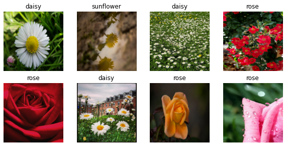
Build Model
First we need to normalize our images between 0 and 1. For this we can devide by 255 and can get required results.
# keras preprocessing normalization
normalization_layer = layers.experimental.preprocessing.Rescaling(1./255)

# Normalize dataset
normalized_ds = train_ds.map(lambda x, y: (normalization_layer(x), y))
image_batch, labels_batch = next(iter(normalized_ds))
Now we build a simple deep learning model for classification. We will use input of 180x180 as defined in above variable. We are also using preprocessing layer to rescale images between 0 and 1.
from keras.layers import Conv2D, MaxPooling2D
from keras.layers import Activation, Dropout, Flatten, Dense

model = Sequential()
model.add(layers.experimental.preprocessing.Rescaling(1./255, input_shape=(img_size[0], img_size[1], 3)))
model.add(Conv2D(32, (3, 3), activation="relu"))
model.add(MaxPooling2D())

model.add(Conv2D(64, (3, 3), activation='relu'))
model.add(MaxPooling2D())

model.add(Conv2D(128, (3, 3), activation='relu'))
model.add(MaxPooling2D())

model.add(Flatten())  # this converts our 3D feature maps to 1D feature vectors
model.add(Dense(256, activation="relu"))
model.add(Dense(3))
As we are training a multiclass classifier, so we will use loss function as Sparse Categorical Crossentropy and for optimizer we are using adam.
model.compile(
    optimizer='adam',
    loss=tf.keras.losses.SparseCategoricalCrossentropy(from_logits=True),
    metrics=['accuracy']
)
Train Model
Now we can train model using training data and model we build in upper steps. We can train model for 10 epochs to check how it train on dataset and will also check its performance using validation dataset. We are also saving model history to variable which then we can use to display train and test accuracy.
epochs=10
history = model.fit(
    train_ds, # training dataset
    validation_data=val_ds, #testing dataset
    epochs=epochs #no of epochs
)
Show Loss and Accuracy
We can use matplotlib to plt both training and validation loss and accuracy to check how model has result on train and validation dataset.
# show training and validation loss
plt.plot(range(epochs), history.history['loss'], label="Training Loss")
plt.plot(range(epochs), history.history['val_loss'], label="Validation Loss")
plt.title("Training and validation loss")
plt.xlabel("Epochs")
plt.legend(loc="upper right")
plt.ylabel("Loss")
plt.show()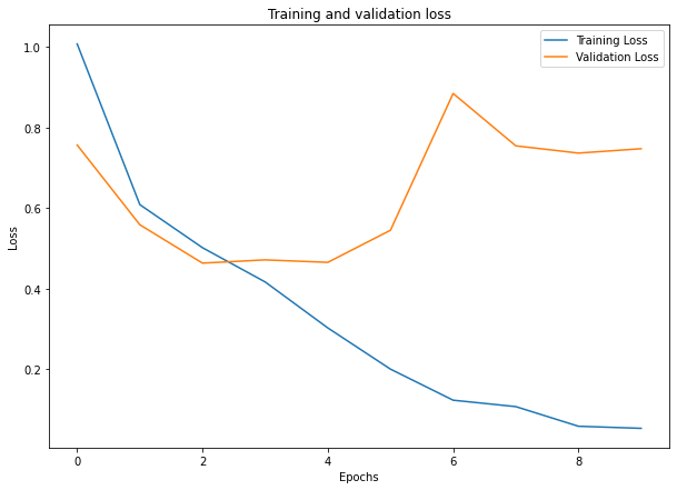
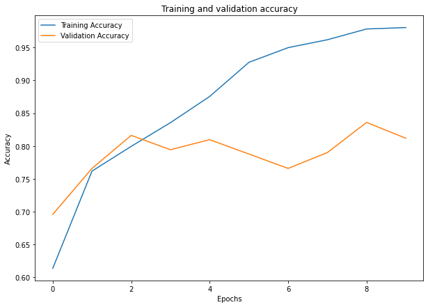
Training and validation accuracy
# show training and validation accuracy
plt.plot(range(epochs), history.history['accuracy'], label="Training Accuracy")
plt.plot(range(epochs), history.history['val_accuracy'], label="Validation Accuracy")
plt.title("Training and validation accuracy")
plt.xlabel("Epochs")
plt.legend(loc="upper left")
plt.ylabel("Accuracy")
plt.show()